Functional trangle solver

由於要加入速度與加速度的計算，因此決定由三角形的 solver 下手，透過 SymPy 模組協助解題，獲得 x 和 y 軸的分量。

編寫概念類似 PMKS 將方程式存起來，因此每個點都會先獲得一個位置函式，接收數值為角速度 ω 與時間 t：

$$f_{x,y}(\omega,t)$$

首先要定義幾個類型方便計算：

from sympy import pi, sqrt, cos, sin, acos, asin, diff, lambdify
from sympy.abc import w, t

class Coordinate:
    def __init__(self, x, y):
        self.x = x
        self.y = y

    #兩座標距離
    def distance(self, p):
        '''
        Coordinate p
        '''
        return sqrt((p.x - self.x)**2 + (p.y - self.y)**2)

    #兩座標與水平軸夾角
    def m(self, p):
        '''
        Coordinate p
        '''
        return asin((p.y - self.y)/self.distance(p))

    #若分量為 SymPy 函式，將其 Lambda 化回傳
    @property
    def functions(self):
        return (
            lambdify((t, w), self.x),
            lambdify((t, w), self.y))

class FunctionBase:
    '''
    Input Coordinate should get from position function.
    '''

    #位置方程式
    @property
    def p(self):
        return Coordinate(self.pxFunc, self.pyFunc)

    #速度方程式：微分 1 次
    @property
    def v(self):
        return Coordinate(diff(self.pxFunc, t), diff(self.pyFunc, t))

    #加速度方程式：微分 2 次
    @property
    def a(self):
        return Coordinate(diff(self.pxFunc, t, 2), diff(self.pyFunc, t, 2))

    #急跳度方程式：微分 3 次
    @property
    def j(self):
        return Coordinate(diff(self.pxFunc, t, 3), diff(self.pyFunc, t, 3))

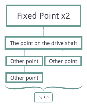
用兩個固定點可以得到繞行旋轉軸的點座標，接著再構建出其他點的位置。

PLAP

由於輸入項目由角度取代成代數，之前的 PLAP 函式改為 PL 函式，輸入連桿與軸端的座標即可。

這裡採用的是圓周運動公式：

$$\left | \vec{x} \right | = r\, cos\, \theta$$ $$\left | \vec{y} \right | = r\, sin\, \theta$$

Python 程式：

class pl(FunctionBase):
    def __init__(self, A, L):
        self.pxFunc = A.x+L*cos(w*t)
        self.pyFunc = A.y+L*sin(w*t)

PLLP

使用底邊夾角與餘弦定理得到座標。

$$\alpha = sin^{-1}(\frac{y_{B}-y_{A}}{\sqrt{(x_{B}-x_{A})^{2}+(y_{B}-y_{A})^{2}}})$$ $$\beta = cos^{-1}(\frac{L^{2}+L_{b}^{2}-R^{2}}{2\times L\times L_{b}})$$

正向：

$$x = x_{A}+L\, cos(\alpha+\beta)$$ $$y = y_{A}+L\, cos(\alpha+\beta)$$

反向：

$$x = x_{A}+L\, cos(\alpha-\beta)$$ $$y = y_{A}+L\, cos(\alpha-\beta)$$

Python 程式：

class pllp(FunctionBase):
    def __init__(self, A, L, R, B, reverse=False):
        alpha = A.m(B)
        base = A.distance(B)
        beta = acos((L**2 + base**2 - R**2)/(2*L*base))
        if reverse:
            self.pxFunc = A.x+L*cos(alpha-beta)
            self.pyFunc = A.y+L*sin(alpha-beta)
        else:
            self.pxFunc = A.x+L*cos(alpha+beta)
            self.pyFunc = A.y+L*sin(alpha+beta)

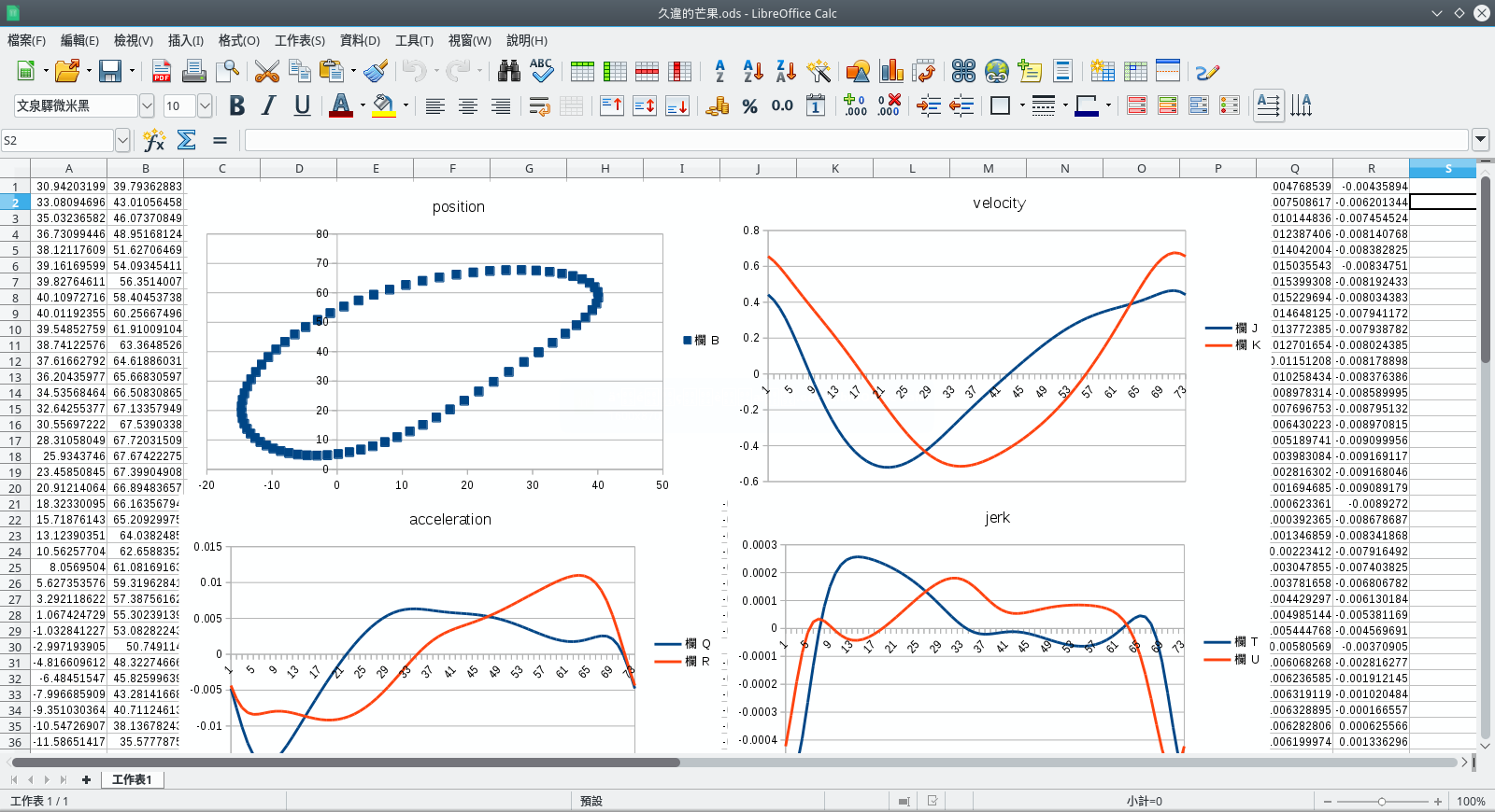
套入四連桿範例

應用到標準曲柄搖桿範例後，可以繪出四者的曲線圖。

通過 solver 這個函式輸入連桿參數：

def solver(mechanism, progress=False):
    results = []
    resultCount = len(mechanism)
    for i, e in enumerate(mechanism):
        if len(e)==2:
            foo = pl(*e)
            results.append(foo)
        else:
            e = list(e)
            if type(e[0])==int:
                e[0] = results[e[0]].p
            if type(e[3])==int:
                e[3] = results[e[3]].p
            foo = pllp(*e)
            results.append(foo)
        if progress:
            print("{} / {}".format(i+1, resultCount))
    return results

最後會回傳一組函式物件，可以透過 FunctionBase 和 Coordinate 類型的方法取值。

p0 = Coordinate(0, 0)
p1 = Coordinate(90, 0)
results = solver([
        (p0, 35.), #p2
        (0, 70., 70., p1), #p3
        (0, 40., 40., 1), #p4
], progress=True)

W = pi/180 #rad/s
for T in range(0, 360+1, 5):
    xfun, yfun = results[2].p.functions
    print("{}\t{}".format(xfun(T, W), yfun(T, W)))

亦可使用 matplotlib 繪出資料。

W = pi/180 #rad/s
plot = []
for T in range(0, 360+1, 5):
    plot.append((xfun(T, W), yfun(T, W)))
import matplotlib.pyplot as plt
plt.plot(plot)
plt.show()

不過反覆測試之後，發現竟然沒辦法套用原本八連桿的配置。

這方面還在解決中，看看是輸入方面還是解題方程式哪裡出了問題。

Pyslvs 開發進度 - 08/25

Functional trangle solver

PLAP

PLLP

套入四連桿範例

Comments